A Water Balancing Act: Water Balances Highlight the Benefits of Community-Based Adaptive Management in Northern New Mexico, USA

Abstract

Quantifying groundwater recharge from irrigation in water-scarce regions is critical for sustainable water management in an era of decreasing surface water deliveries and increasing reliance on groundwater pumping. Through a water balance approach, our study estimated deep percolation (DP) and characterized surface water and groundwater interactions of two flood-irrigated fields in northern New Mexico to evaluate the regional importance of irrigation-related recharge in the context of climate change. DP was estimated for each irrigation event from precipitation, irrigation input, runoff, change in soil water storage, and evapotranspiration data for both fields. Both fields exhibited positive, statistically significant relationships between DP and total water applied (TWA), where one field exhibited positive, statistically significant relationships between DP and groundwater level fluctuation (GWLF) and between GWLF and total water applied. In 2021, total DP on Field 1 was 739 mm, where 68% of irrigation water applied contributed to DP. Field 2′s total DP was 1249 mm, where 81% of irrigation water applied contributed to DP. Results from this study combined with long-term research indicate that the groundwater recharge and flexible management associated with traditional, community-based irrigation systems are the exact benefits needed for appropriate climate change adaptation.

1. Introduction

Over 50% of the world’s freshwater resources for human use and consumption rely on river discharge that can be greatly impacted by long-term changes in precipitation and temperature such as those caused by climate change, particularly in snow-dominated regions [1]. Much of the western United States depends on precipitation falling in the winter in mountainous regions as snow and subsequently released slowly as snowmelt throughout the following spring and summer seasons. However, long-term changes in temperature and precipitation are already affecting these crucial water resource systems by decreasing the maximum snowpack accumulation, shifting the timing of runoff to arrive earlier, and impacting the volume of river discharge [2,3] with changes amplified by a lack of reservoir storage [4]. More specifically, snow-dominated basins in the mid-high latitudes are the most vulnerable to the impacts of warming climates where maximum runoff is expected to arrive one month earlier by 2050 in the western United States [1].

For example, the Rio Grande and its tributaries are increasingly becoming water stressed due to the warming climate and the increasing demand from users in Colorado, New Mexico, Texas, and Mexico [5]. Rio Grande streamflow is vulnerable as it largely depends on snowpack conditions which are projected to decrease and melt earlier in the future [6,7,8,9]. This surface water resource must serve industrial, tourist, residential, agricultural, ecologic, and economic needs in the USA (e.g., Colorado, New Mexico, Texas) and Mexico. Under current climate conditions, New Mexico does not have water to spare between all users [10].

Oftentimes, agricultural sectors are the largest users of water and face greater pressure to develop new water management strategies to help non-agricultural sectors cope with future water scarcity caused by warming temperatures and climate uncertainty [11,12]. In New Mexico in 2015, irrigated agriculture accounted for 76% of total water use, 53% from surface water and 47% from groundwater. Flood irrigation is used on 45% of all irrigated fields in New Mexico [13].

Common water delivery systems for flood irrigation in New Mexico are acequia networks which face many socio-environmental challenges. First introduced to northern New Mexico in the 16th century, acequias are gravity-driven water delivery networks and also serve as the basis of community-managed water governance systems [14,15]. While acequias have many beneficial hydrologic (e.g., aquifer recharge) and social attributes (e.g., water sharing) that foster resilience [16], these ancient water systems still face the challenge of long-term, regional drought and difficult water policy [17,18]. Questions are continually raised at acequia irrigator meetings and posed to researchers regarding what the “right” management strategies are: Should we line the canals? Should we switch to drip? Should we pump groundwater? Irrigators find themselves stuck between cultural norms of propagating generational knowledge of traditional irrigation methods and pressures from decreasing water availability and outside agencies to modernize water delivery systems and maximize irrigation efficiency.

Agricultural irrigation practices involving surface water can cause percolation and groundwater recharge that significantly impact groundwater resources on regional scales [12,19,20,21,22]. A study by Bouimouass et al. (2020) focused on the acequia counterpart in Morocco—seguias—and concluded that flood irrigation of diverted surface water resulted in the dominant recharge process in mountain front landscapes [23]. Other studies from large agricultural drainages in China found that approximately 70% of applied flood irrigation water in maize fields recharged the groundwater during the growing season [24], and seepage from both irrigation canals and deep percolation (DP) from irrigation contributed to more than 90% of total annual shallow groundwater recharge [12]. Additionally, in a large traditional agricultural basin in Italy, irrigation water delivered through a system of canals provided 55 to 88% of groundwater recharge [25]. DP is the amount of water that travels below the effective root zone (ERZ) that can potentially reach the shallow aquifer [26]. One of our previous studies conducted in northern New Mexico showed that peak groundwater level response fluctuated up to 380 mm 8 to 16 h after the onset of flood irrigation [27], where another estimated 16% of unlined irrigation canal flows seeped into the subsurface, causing the water table to rise 1 to 1.2 m [28]. Additionally, annual shallow aquifer recharge ranged from 1044 to 1350 mm on a valley scale [22]. In these cases, DP from flood irrigation was a significant source of recharge to shallow groundwater. DP below the vegetative root zone can provide very important hydrologic and ecosystem benefits in irrigated valleys of semiarid and arid regions.

Conversely, groundwater may display evidence of interactions with surface water. As irrigation water infiltrates into the shallow aquifer, this DP can contribute groundwater return flows to the river. In northern New Mexico, this interaction is of particular interest considering DP can serve as temporary subsurface storage which provides delayed return flow during low-flow periods [22,29,30]. This serves as an important possible buffer for changing peak runoff timing associated with climate variability [19].

Considering interacting surface water and groundwater as one resource is essential for optimal protection of watersheds, sustaining water resources, and furthering integrated groundwater management [20,31]. This is critical within irrigation districts that are increasingly relying on pumping groundwater for agricultural and municipal uses, which can lead to the disconnection of surface water and groundwater [32]. More recently, groundwater recharge via flooding fields is becoming a more common conservation practice [33,34].

It is necessary to properly quantify aquifer recharge and foster an accurate understanding of DP and surface water and groundwater interactions in water-limited regions [35]. The water balance method is a technique commonly used to quantify groundwater recharge and characterize surface water and groundwater interactions [19,22,26,36,37]. Components of the water balance are precipitation, irrigation water applied, runoff, change in soil water storage, and evapotranspiration, where DP is unknown and calculated by the difference of these inputs and outputs [26].

Our first objective was to characterize and compare surface water and groundwater interactions and shallow aquifer response to irrigation events in flood-irrigated forage grass fields located within the same irrigated valley in northern New Mexico by estimating DP below the root zone with a water balance approach. Our second objective was to justify community-based adaptive management in the context of climate change by relating field-scale findings to regional climate change literature. The innovative approach of identifying tightly coupled objectives reflected the unique, tightly coupled natural and human irrigation system our study focused on. While cultivating a better understanding of available surface water resources is extremely important, irrigators and policy makers must also understand the effects of irrigation techniques on groundwater and surface water availability for downstream users [31]. Previous studies have quantified and compared DP across several crop fields, soil types, and valleys in northern New Mexico, USA [22,26]; however, more field observations of DP are needed to expand these studies from field-scale to valley or regional scales. We hypothesized that: (1) DP and total water applied and DP and groundwater response would be positively related on both fields; and (2) DP and total water applied would be significantly different across both study fields.

2. Materials and Methods

2.1. Study Area

This study was conducted on two acequia-irrigated fields in the Rio Hondo agricultural valley in northern New Mexico, USA. The Rio Hondo watershed drains an area of 185 km² [38] and is located 2200 m above sea level [18]. Snowmelt from the Sangre de Cristo Mountains serves as the Rio Hondo’s main source of water and drains to the Rio Grande. Located in a semiarid steppe climate, 50% of the precipitation in this region falls during the monsoon season from June to September [39] with an annual average of 300 mm∙year⁻¹ [40]. The primary settlements in the Rio Hondo Valley are Valdez and Arroyo Hondo. The agricultural activity in the Rio Hondo watershed is small-scale in nature. Eight canals divert water from the Rio Hondo and deliver irrigation water to approximately 1161 ha through a system of branching acequias [38]. Typical crops include grasses (Mostly Phleum pretense, Poa pratensis), alfalfa (Medicago sativa), orchards (e.g., plums, apples, apricot), and vegetables (e.g., squash, beets, greens, onions, radishes, etc.) [41].

Located in the community of Valdez within the Rio Hondo watershed, the first study field (F1) was approximately 27 km north of Taos, New Mexico, USA and covered 2.51 ha (Figure 1a). The main crops grown on the field were grasses, alfalfa, and clovers. The second study field (F2), located in the community of Arroyo Hondo within the Rio Hondo watershed, was approximately 20 km north of Taos, New Mexico (Figure 1b) and covered 1.62 ha. The main crops growing were grasses, alfalfa, and clovers.

Soil Physical Properties

Of F1′s total 2.51 ha, 2.35 ha were Manzano clay loam, and 0.16 ha were Loveland clay loam soil types. For the Manzano clay loam soil, slope values typically range from 3 to 5%, the soil is well-drained with medium runoff, average depth to the water table is more than 2 m, and a typical soil profile is clay loam for the top 1.5 m. For the Loveland clay loam soil, slope values typically range from 0 to 3%, the soil drains poorly and has a high runoff class, average depth to the water table is 0.15 to 0.46 m, and a typical soil profile is clay loam for the top 0 to 0.23 m, sandy clay loam for the middle 0.23 to 0.53 m, and very gravelly sand for the bottom 0.53 to 1.52 m [42].

Of F2′s total 1.62 ha, 1.29 ha were Fernando silt loam, 0.24 ha were Fernando clay loam, and 0.08 ha were from the Sedillo–Silva association. The Fernando silt loam slope values typically range from 0 to 7% and are well drained with medium runoff. The average depth to the water table is greater than 2 m, and a typical soil profile is silt loam for the top 0 to 0.20 m, silty clay loam for the middle 0.20 to 0.91 m, and silt loam for the bottom 0.91 to 1.52 m. The Fernando clay loam generally has slope values from 3 to 5%, is well drained with medium runoff, depth to the water table is more than 2 m, and a typical soil profile is clay loam for the top 0 to 0.18 m, silty clay loam for the middle 0.18 to 0.64 m, and silty loam for the bottom 0.64 to 1.52 m. The Sedillo–Silva association soil typically has a slope of 10 to 25%, is well drained with high runoff, depth to the water table is greater than 2 m, and a typical soil profile is very gravelly loam for the top 0 to 0.08 m, gravelly clay loam for the middle 0.08 to 0.28 m, and very cobbly sandy loam for the bottom 0.28 to 1.52 m [43].

Soil bulk density varied between the two fields, whereas soil texture remained relatively consistent (

Table 1. Soil physical properties for the two field sites from manual soil sample collection (see Section 2.2.3). Laboratory analysis determined soil bulk density, soil particle distribution, and soil texture for each sensor depth in the soil profile. Values for each soil depth represent the averaged value between the two soil-monitoring stations on each field.

Field	Soil Depth (m)	Bulk Density (Mg∙m−3)	Sand (%)	Silt (%)	Clay (%)	Soil Texture
F1	0.2	1.46 × 109	72.6	17.6	9.90	Sandy loam
	0.5	1.35 × 109	55.6	27.5	16.9	Sandy clay loam
	0.8	1.23 × 109	51.7	31.5	16.9	Sandy clay loam
F2	0.2	1.19 × 109	60.6	27.4	12.0	Sandy clay loam
	0.5	1.26 × 109	59.6	32.5	7.90	Sandy clay loam
	0.8	1.27 × 109	57.5	32.4	10.0	Sandy clay loam

). For F1, bulk density ranged from 1.46 × 10⁹ Mg∙m⁻³ in the topsoil to 1.23 × 10⁹ Mg∙m⁻³ toward the bottom of the soil profile. Within the field F2 soil profile, bulk density ranged from 1.19 × 10⁹ Mg∙m⁻³ to 1.27 × 10⁹ Mg∙m⁻³ from top to bottom. Soil texture was sandy clay loam for all soil depths except the top layer of the F1 soil profile which was sandy loam. Soil texture components exhibited the same trends through the soil profile for sand and silt but differed for clay. Sand content decreased, and silt content increased toward the bottom of the soil profile for both fields, while clay content increased in F1 and decreased in F2 (Table 1).

2.2. Field Data Collection

We monitored various parameters at both study sites to calculate DP using a water balance approach for irrigation events over the 2020 and 2021 irrigation seasons. The water balance method was an appropriate approach for our study given our goals of estimating recharge for individual irrigation events within an irrigation season and subsequently relating our findings to community adaptive management and climate change. DP is the water that infiltrates into the subsurface, past the ERZ. ERZ varies depending on crop root development, effective soil depth, soil fertility or fertility management, and soil physical properties [44]. We recorded ERZ measurements of root systems at each site during soil volumetric water content (θ) sensor installation where F1 ERZ was 0.51 m and F2 ERZ was 0.53 m. Data collected throughout the 2020 and 2021 irrigation seasons returned a groundwater recharge estimate for each irrigation event through a field-scale water balance approach:

DP = PPT + IRR − RO − ∆S − AET

(1)

where PPT is the amount of rainfall during the time interval (mm), IRR is irrigation water applied during the time interval (mm), RO is the amount of irrigation runoff during the time interval (mm), ∆S is the change of storage or change in θ during the time interval (mm), and AET is the actual evapotranspiration during the time interval (mm). The time interval for each irrigation event begins with the onset of irrigation and extends to 24 h after the end of the irrigation water delivery to achieve an assumed state of field capacity.

2.2.1. Precipitation

Precipitation falling on the study sites during the irrigation season was mainly rainfall measured by weather stations on each field. Both weather stations were equipped with a tipping bucket rain gauge (ClimaVUE50, Campbell Scientific, Inc.; Logan, UT, USA) programmed to record incremental precipitation every five minutes.

2.2.2. Irrigation Inflow and Outflow

Property owners and field managers for both fields used acequia-delivered surface water to flood irrigate throughout the growing season and decided to irrigate based on water allocations, environmental conditions, and crop needs. Surface water is diverted from the acequia onto fields through a series of wooden and metal headgates depending on the size and orientation of the field with respect to the acequia. F1 had five irrigation inflow monitoring stations and one irrigation outflow station. F2 had one irrigation inflow monitoring station and one irrigation outflow station. Rectangular Samani–Magallanez flumes [45] installed at inflow and outflow locations, each equipped with a CS451 pressure transducer and a CR300 datalogger (Campbell Scientific, Inc.; Logan, UT, USA) and programmed to record water level at five-minute increments measured IRR and RO on each field.

2.2.3. Soil Water Content and Physical Properties

Derived from soil volumetric water content data, the change in storage was determined as:

$$\Delta S={\displaystyle \sum }_{i=1}^n{\left({\theta }_2-{\theta }_1\right)}_i\Delta d_i$$

(2)

where n is the number of layers represented by a soil sensor in the ERZ profile, θ₁ is the soil volumetric water content at the onset of irrigation (m³∙m⁻³), θ₂ is the soil volumetric water content 24 h after irrigation ends or the average soil volumetric water content at field capacity (m³∙m⁻³), and ∆d_i is the soil layer thickness (mm). Equation (2) converted θ at each sensor location to the amount of water (mm) held in the ERZ.

Each field had two monitoring stations measuring θ. At each station, a CR300 datalogger and three horizontally placed CS655 (Campbell Scientific, Inc.; Logan, UT, USA) soil sensors were arranged vertically in the ERZ at depths of 0.2 m, 0.5 m, and 0.8 m and recorded changes in θ every minute and averaged data at 30-min increments.

Soil samples collected while installing the sensor network underwent laboratory analysis to determine soil texture and bulk density. Three soil cores were collected at each sensor depth on the opposite wall of the pit where sensors were installed with a split soil core sampler and analyzed with the Blake and Hartge bulk density method [46] and the Gee and Bauder hydrometer method to determine soil texture [47].

2.2.4. Evapotranspiration

We used the following equation to calculate the amount of actual evapotranspiration (AET):

AET = K_cET₀

(3)

where ET₀ is the total evapotranspiration (mm) calculated with the Penman–Monteith equation programmed into a CR1000 datalogger (Campbell Scientific, Inc.; Logan, UT, USA). The Penman–Monteith equation outperforms others by including more factors that influence crop water loss (e.g., absorbed radiant energy, wind, atmospheric vapor deficit) and is therefore expected to provide more accurate estimates [48]. Post-processing the ET₀ values with crop coefficient (K_c) values calculates AET. We used crop coefficient curves for grass at different stages of the growing season presented in a previous study that took place near our study area [49] (p. 151). ET₀ values were recorded, and AET values were calculated for hourly data.

2.2.5. Groundwater Level

Three monitoring wells equipped with water level loggers (HOBO Logger U20-001-01, Onset; Bourne, MA, USA) recorded water table fluctuations on each field. All monitoring wells on F1 were steel drive-point wells 2 to 3 m deep. Two of these wells were installed by previous researchers [26]. We installed two steel drive-point wells 2 to 3 m deep on F2 and used the landowner’s residential drinking well that was 13 m deep for the third monitoring well. This residential well has been used for long-term groundwater monitoring, where the data clearly show groundwater level response to the irrigation season.

The groundwater level data helped characterize shallow aquifer response to DP from irrigation inputs. Calculated for each irrigation event, groundwater level fluctuation (GWLF) (mm) was the difference between groundwater level prior to the irrigation onset (averaged over the 6 h prior to the irrigation onset) and maximum water level rise until the following irrigation event. Negative GWLF values indicate declining groundwater levels.

2.3. Statistical Analyses

Specific parameters that characterize surface water and groundwater interactions underwent linear regression and ANOVA statistical analyses to delineate any significant relationships within and across fields. Linear regression models evaluated and compared interactions between total water applied (TWA = IRR + PPT − RO) and DP, DP and GWLF, TWA and GWLF. ANOVA analyses identified significant differences in means between the two study fields and different stations. Differences were considered significant at α = 0.05. The 2020 irrigation season data collection only spanned mid-June through October (partial season), whereas the 2021 irrigation season data collection spanned April through October (complete season). Therefore, only 2021 data were included in the statistical analysis and presented in the Results section of this paper for optimal scientific consistency and comparability.

3. Results

3.1. Irrigation Events and Deep Percolation Estimates

The number of irrigation events and DP varied between both fields over the 2021 irrigation season (

Table 2. DP results calculated with the water balance method for each irrigation event in the 2021 irrigation season for F1. This table shows the total time of irrigation, change in θ (∆S), total irrigation water applied (IRR), tailwater runoff (RO), total precipitation (PPT), and total AET from the beginning of each irrigation event to 24 h after the end of irrigation. DP estimates that resulted in negative values likely due to large ∆S values were considered to be 0, where no recharge occurred.

Date	Irrigation Duration (h)	∆S (mm)	IRR (mm)	RO (mm)	PPT (mm)	AET (mm)	DP (mm)
27 April 2021	49	55	158	0	0	8	94
4 May 2021	49	11	185	0	0	11	162
11 May2021	48	105	197	2	0	14	76
18 May 2021	58	−3	138	1	7	13	134
24 May 2021	45	23	235	47	0	18	147
1 June 2021	83	−6	135	0	1	21	122
23 July 2021	70	18	12	0	22	11	5
31 July 2021	165	129	34	0	5	22	0
Average	71	42	137	6	4	15	92

and

Table 3. DP results calculated with the water balance method for each irrigation event in the 2021 irrigation season for F2. This table shows the total time of irrigation, change in θ (∆S), total irrigation water applied (IRR), tailwater runoff (RO), total precipitation (PPT), and total AET from the beginning of each irrigation event to 24 h after the end of irrigation. DP estimates that resulted in negative values likely due to large ∆S values were considered to be 0, where no recharge occurred.

Date	Irrigation Duration (h)	∆S (mm)	IRR (mm)	RO (mm)	PPT (mm)	AET (mm)	DP (mm)
16 April 2021	70	46	313	0	8	6	270
10 May 2021	5	−1	0	0	0	5	0
10 May 2021	8	−1	5	0	0	1	6
11 May 2021	11	0	2	0	0	6	0
11 May 2021	11	0	2	0	0	0	2
12May 2021	36	3	51	0	0	11	37
13 May 2021	9	0	2	0	0	0	2
14 May 2021	98	164	341	0	22	24	175
18 May 2021	10	−55	1	0	4	2	68
19 May 2021	40	−23	18	0	2	15	27
23 May 2021	2	−3	0	0	0	2	1
24 May 2021	1	−2	1	0	0	4	0
24 May 2021	18	−6	0	0	0	10	0
29 May 2021	33	−5	8	0	0	7	5
31 May 2021	23	−4	3	0	16	7	15
5 June 2021	78	−5	216	3	2	31	189
26 June 2021	112	82	397	8	11	10	308
1 August 2021	58	6	26	0	7	12	15
18 August 2021	7	−3	1	0	0	3	1
18 August 2021	39	−4	39	0	0	6	37
27 August 2021	8	−4	12	0	0	6	10
29 August 2021	18	−4	20	0	0	7	17
8 September 2021	50	−4	70	0	0	11	63
11 September 2021	8	−1	2	0	0	6	0
Average	31	7	64	0	3	8	52

). Eight irrigation events took place on F1 (Table 2). A total of 24 irrigation events took place on F2 (Table 3). The average IRR was 137 mm, and the DP was 92 mm per irrigation event on F1 (Table 2). The average IRR was 64 mm, and the DP was 52 mm per irrigation event on F2 (Table 3). The F1 DP estimates total was 739 mm, where 68% of the IRR contributed to DP (

Table 4. Summary table displaying total number of irrigation events, cumulative IRR, DP, and percent of IRR that contributed to DP for each field over the 2021 irrigation season.

Field	Year	Number of Irrigation Events	IRR (mm)	DP (mm)	Percent DP (%)
F1	2021	8	1093	739	67.7
F2	2021	24	1541	1249	81.1

). For F2, the DP estimates total was 1249 mm, where 81% of the IRR contributed to DP (Table 4).

While annual variability is common due to differing environmental conditions, surface water availability, and irrigation scheduling, monthly irrigation summaries and averages on both fields demonstrate similar ranges of water balance parameters between 2020 and 2021 (

Table 5. Comparison of monthly number of irrigation events, average ∆S, average IRR, average RO, average PPT, average DP, and total DP for F1 and F2 for three months in 2020 and 2021. The months chosen for comparison are July through September because these were the first complete monthly records after data collection began in 2020 (data collection began early-June 2020) to ensure optimal comparability between the two irrigation seasons on both fields.

Field	Month	Number of Irrigation Events	Avg ∆S (mm)	Avg IRR (mm)	Avg RO (mm)	Avg PPT (mm)	Avg AET (mm)	Avg DP (mm)	Sum DP (mm)
F1	July 2020	2	−3	13	0	1	4	12	24
	August 2020	1	−3	31	0	5	10	29	29
	September 2020	0	(no irrigation events)
	July 2021	2	73	23	0	13	16	2	5
	August 2021	0	(no irrigation events)
	September 2021	0	(no irrigation events)
F2	July 2020	0	(no irrigation events)
	August 2020	3	2	11	0	5	7	9	27
	September 2020	2	−1	6	0	0	6	1	3
	July 2021	0	(no irrigation events)
	August 2021	5	−2	19	0	1	7	16	80
	September 2021	2	−3	36	0	0	8	32	63

). On F1 in 2020, DP averaged 12 mm and 29 mm per irrigation event in July and August, respectively, with no irrigations in September. In 2021, the average DP for July was 2 mm with no irrigations in August or September. No irrigations took place on F2 in July in 2020 and 2021. In 2020, F2 DP averaged 9 mm in August and 1 mm in September. In 2021, DP averaged 16 mm in August and 32 mm in September.

The linear regression analysis showed a positive, significant relationship between DP and TWA and TWA-∆S for both F1 (p = 8.37 × 10⁻³ and p = 3.48 × 10⁻⁴, respectively) and F2 (p = 7.88 × 10⁻¹⁶ and p < 2.00 × 10⁻¹⁶, respectively) (

Table 6. Statistics from linear regression models comparing DP and TWA, DP and TWA-∆S, and DP and irrigation duration for irrigation events on each field in 2021. Significant relationships are highlighted by p values with an asterisk (*).

Field	t	R2	p
TWA (mm)
F1	3.86	0.713	8.37 × 10−3 *
F2	16.4	0.925	7.88 × 10−16 *
TWA-∆S (mm)
F1	7.26	0.898	3.48 × 10−4 *
F2	67.9	0.995	<2.00 × 10−16 *
Irrigation duration (h)
F1	−2.12	0.427	0.0787
F2	8.04	0.746	5.42 × 10−8 *

). Previous research in the region found that prior θ significantly impacted DP [50], which is why we included TWA-∆S in the linear regression. Additionally, F2 exhibited a significant positive relationship between DP and irrigation duration (p = 5.42 × 10⁻⁸). ANOVA showed statistically significant differences in the mean irrigation duration and mean number of irrigation events between F1 and F2 (

Table 7. ANOVA tests conducted with the field as the independent variable and different variables of interest as dependent variables to identify significant differences in means between surface water and groundwater interactions and irrigation management across both fields for 2021 irrigation events. Significant differences are highlighted by p values with an asterisk (*).

Dependent Variable	F	R2	p
DP (mm)	1.40	0.0447	0.245
TWA (mm)	2.23	0.0691	0.146
TWA-∆S (mm)	0.811	0.0263	0.375
Irrigation duration (h)	8.17	0.214	7.67 × 10−3 *
Number of irrigation events	9.66	0.244	4.09 × 10−3 *

).

3.2. Shallow Groundwater Response to Irrigation Inputs

GWLF and response to irrigation inputs were observed for both study fields over the 2020 and 2021 irrigation seasons (Figure 2). In 2021 on F1, gw1 GWLF averaged 533 mm, gw2 GWLF averaged 262 mm, and gw3 GWLF averaged 863 mm. The greatest observed GWLF of the F1 monitoring wells was 1699 mm on 11 May 2021 (

Table 8. GWLF (mm) in response to irrigation events in 2021 for all wells on F1 calculated as the difference between groundwater level prior to the irrigation onset (averaged over the 6 h prior to the irrigation onset) and maximum water level rise until the following irrigation event.

Date	GWLF gw1 (mm)	GWLF gw2 (mm)	GWLF gw3 (mm)
27 April 2021	452	0	1549
4 May 2021	1601	55	0
11 May2021	197	781	1699
18 May 2021	1363	280	288
24 May 2021	55	428	1350
1 June 2021	−6	108	618
23 July 2021	320	150	114
31 July 2021	282	290	1282
Average	533	262	863

).

Both study fields exhibited sharp groundwater response to irrigation events and DP (Figure 2). F1 groundwater levels would generally show a moderate decline after the peak GWLF (Figure 2a). F1 gw1, located next to the irrigation canal, maintained more elevated groundwater levels for longer than the other two wells on this field. Gw3 displayed the “flashiest” response to irrigation events and DP both in the rise and fall around the peak GWLF.

F2 groundwater levels—specifically gw2 and gw3—would decline more rapidly following the peak GWLF (Figure 2b). F2 gw1 showed more short-term fluctuation due to pumping water for residences on the property and more gradual rise and fall to the beginning and end of the irrigation season due to its deeper reach, upgradient position, and closer tie to ditch seepage from nearby acequias and water delivery canals rather than irrigation events. On F2, GWLF in gw1 differed from the groundwater response in the other monitoring wells to irrigation events (Figure 2b). This well (gw1) was the landowner’s drinking water well that was 13 m deep and located upgradient of the irrigated field (Figure 1). GWLF from F2 gw1 levels were likely related to acequia flow as opposed to irrigation events. The main acequia flowed along the south border of the property, and the intermediate ditch that delivered water from the acequia onto F2 flowed next to gw1, so ditch seepage from delivery canals likely supplied this well. F2 gw1 GWLF averaged 167 mm in 2021. For the other F2 monitoring wells gw2 and gw3, GWLF averaged 210 mm and 272 mm, respectively. The greatest observed GWLF of the F2 monitoring wells was 1697 mm on 14 May 2021 (

Table 9. GWLF (mm) in response to irrigation events in 2021 for all wells on F2 calculated as the difference between groundwater level prior to the irrigation onset (averaged over the 6 h prior to the irrigation onset) and maximum water level rise until the following irrigation event.

Date	GWLF gw1 (mm)	GWLF gw2 (mm)	GWLF gw3 (mm)
16 April 2021	876	602	1677
10 May 2021	100	7	42
10 May 2021	87	21	87
11 May 2021	76	141	129
11 May 2021	30	132	103
12May 2021	278	275	288
13 May 2021	53	−3	20
14 May 2021	242	1697	969
18 May 2021	3	−45	−23
19 May 2021	254	−40	47
23 May 2021	40	−7	−9
24 May 2021	−35	−8	−15
24 May 2021	57	3	1
29 May 2021	198	−1	−4
31 May 2021	164	30	33
5 June 2021	362	418	795
26 June 2021	247	1179	1204
1 August 2021	93	140	345
18 August 2021	41	0	43
18 August 2021	168	220	430
27 August 2021	30	96	147
29 August 2021	250	145	76
8 September 2021	368	3	28
11 September 2021	33	33	106
Average	167	210	272

).

Linear regression statistical analysis identified any significant relationships between DP and GWLF of each monitoring well as well as TWA and GWLF of each monitoring well for both study fields (

Table 10. Statistics from linear regression models comparing GWLF and DP as well as GWLF and TWA for all monitoring wells on each field from data collected over the 2021 irrigation season. Significant relationships are highlighted by p values with an asterisk (*).

	GWLF gw1 (mm)			GWLF gw2 (mm)			GWLF gw3 (mm)
	t	R2	p	t	R2	p	t	R2	p
DP (mm)
F1	1.19	0.190	0.280	−0.252	0.0105	0.810	−0.426	0.0294	0.685
F2	4.60	0.490	1.40 × 10−4 *	5.78	0.603	8.09 × 10−6 *	11.5	0.858	8.77 × 10−11 *
TWA (mm)
F1	0.540	0.0464	0.608	0.720	0.0795	0.499	0.639	0.0638	0.546
F2	3.93	0.413	7.08 × 10−4 *	10.3	0.828	7.37 × 10−10 *	11.4	0.856	9.91 × 10−11 *

). No significant relationships were identified between GWLF and DP nor GWLF and TWA for any F1 monitoring wells. This is likely related to the land manager’s use of several headgates spread out along the southern field border used at different times unevenly applying irrigation water. All wells on F2 exhibited positive significant relationships between GWLF and DP, and GWLF and TWA (Table 10). However, F2 gw1 GWLF was likely related to acequia flow and ditch seepage rather than irrigation events due to its upgradient position.

Figure 3 provides a visualization of how the groundwater level data from the three monitoring wells compare across the two study fields. The greatest variation is apparent between gw1 on F1 and F2 because the well on F2 is a residential drinking well and is much deeper (see Section 2.2.5 for more detailed metrics regarding the groundwater monitoring wells included in this study).

4. Discussion

Our results showed both fields have significant relationships between DP and TWA and between DP and TWA-∆S (Table 6). One field, F2, exhibited significant relationships between DP and irrigation duration (Table 6), GWLF and DP, and GWLF and TWA (Table 10). Antecedent soil moisture and soil conditions are particularly important factors to consider when discussing DP. More irrigation water is needed to saturate the ERZ when antecedent soil moisture is low or at times of greater plant water use which results in potentially less groundwater recharge from a given amount of irrigation water applied. DP was not significantly different when compared across both fields. The only significant differences when comparing irrigation events and DP estimates across both fields were irrigation duration and the number of irrigation events (Table 7). These results indicate that surface water and groundwater are tightly connected in this area, but variation in DP and groundwater response exists between land managers and fields due to differing irrigation practices.

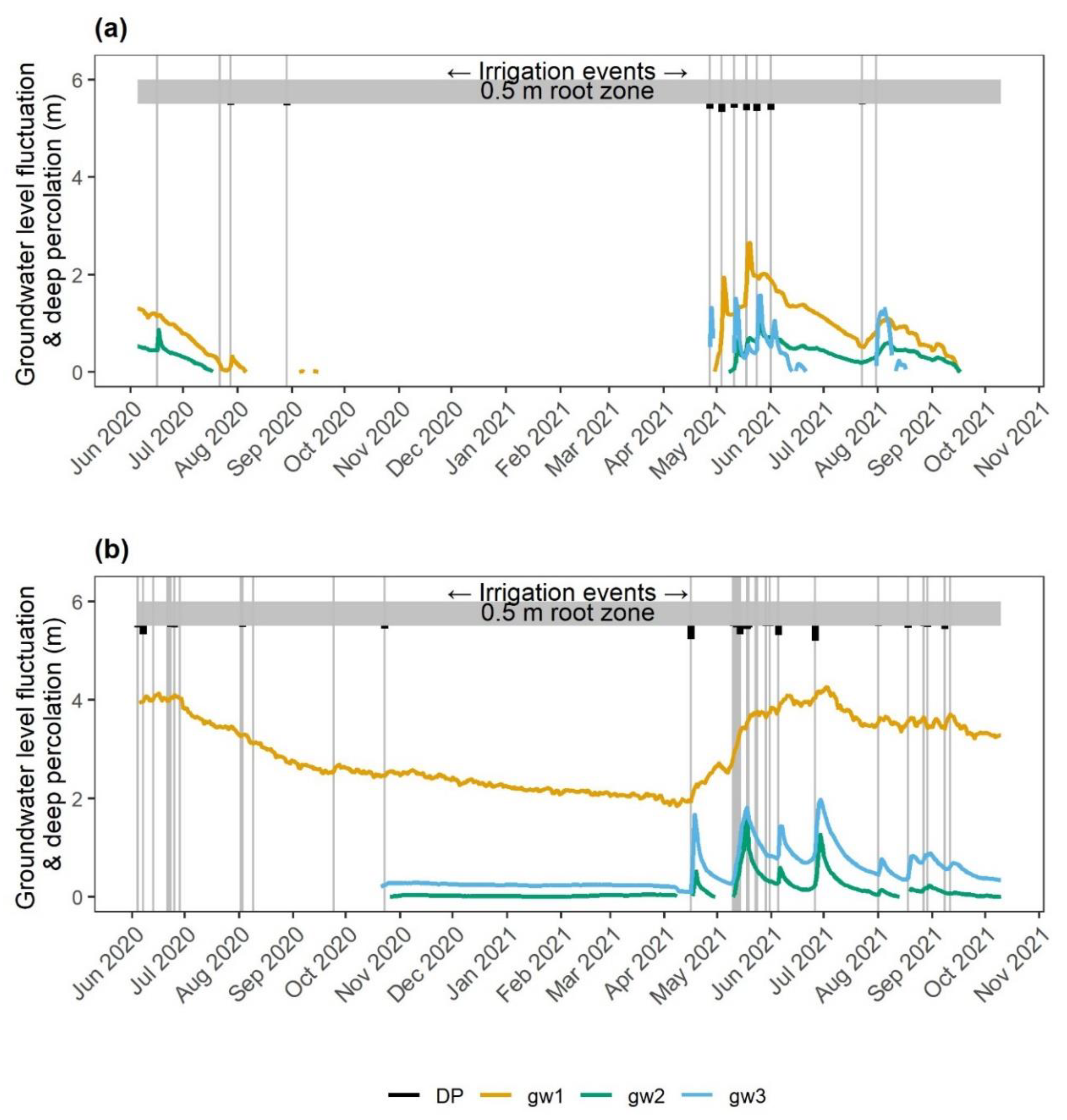
Although we only report data and results from the 2021 irrigation season, our data collection began in June 2020. When comparing monthly averages and totals for months with complete records for both 2020 and 2021, several patterns emerge regarding irrigation scheduling, average ∆S, and average DP (Table 5). F1 irrigation frequency tapered off toward the end of the irrigation season for both 2020 and 2021, while F2 irrigation frequency increased toward the end of the season. Average ∆S was constant between the two fields over both years of data collection, ranging from −3 to 2 mm with a notably large value for F1 in July 2021 (73 mm) as an outlier perhaps related to frequent rainfall that occurred around that time of year and uneven irrigation water application. On F1, the average DP ranged from 2 to 29 mm over 2020 and 2021. Similarly, the F2 average DP ranged from 1 to 32 mm. These patterns help validate our water balance results (Table 2 and Table 3) by demonstrating consistent and comparable water balance components and DP estimates across both fields over 2020 and 2021.

Previous acequia research in northern New Mexico forage fields that also used water balance methodology to estimate DP reflects similar results (

Table 11. A comparison of how our DP estimates compare to similar studies that used a water balance approach to estimate DP in forage grass fields in northern New Mexico.

Study	Location & Year	Average DP per Irrigation Event (mm)	Sum DP over Irrigation Season (mm)	Percent DP over Irrigation Season (%)
Ochoa et al. (2013)	Alcalde 2005	107	533	46
Ochoa et al. (2013)	Alcalde 2006	119	476	48
Gutiérrez-Jurado et al. (2017)	Rio Hondo (F1) 2013	53	531	51
Gutiérrez-Jurado et al. (2017)	Alcalde 2013	55	382	39
Gutiérrez-Jurado et al. (2017)	El Rito 2013	77	462	31
Conrad et al. (this paper)	Rio Hondo (F1) 2021	92	739	68
	Rio Hondo (F2) 2021	52	1249	81

), illustrating that we appropriately captured acequia surface water and groundwater interactions and irrigation practices. Our results reflected the greatest DP season totals (739 and 1249 mm) and the greatest percentage of IRR that contributed to DP (68 and 81%), critically filling in the range of possible seasonal DP values and characteristics by refining our understanding of acequia irrigation-related recharge in the context of long-term field data collection in northern New Mexico.

Observations and projections of changing climate and snowmelt dynamics within the Rio Grande Basin—specifically the Upper Rio Grande headwaters region—are of particular interest to researchers and stakeholders due to the reliance of downstream users on snowmelt-dominated subbasins to meet water availability needs. For example, streamflow at Fort Quitman, Texas, USA has decreased 95% relative to the river’s native streamflow [51]. In the Colorado River Basin, temperature-driven “hot droughts” have been connected to increased sublimation of snow which results in less runoff from a given snowpack [52]. Similarly, the interannual variability of streamflow related to snow water equivalent (SWE) has decreased by 40% in the Upper Rio Grande Basin, indicating that the connection between peak SWE and runoff volume is substantially weaker [7]. This drift between SWE and runoff is particularly critical because a large portion—50 to 75%—of the Rio Grande streamflow is sustained by seasonal snowpack accumulation [53]. Through paleoclimate reconstructions published in 2017, researchers identified a 30-year declining trend in runoff ratio since the 1980s which appeared unprecedented in the context of the last 440 years [54]. Observed, historical mean winter and spring temperatures have significantly increased in the Upper Rio Grande Basin [7], and temperatures rose at an alarming rate of 0.4 °C per decade from 1971 through 2011, informing temperature predictions of a 2 to 3 °C increase in average temperature by the end of the 21st century [8]. The SWE on April 1 has significantly decreased by 25% [7], where the mean melt season snow covered area is predicted to decrease 57 to 82%, and peak flow is predicted to arrive 14 to 24 days earlier than usual [6].

The combination of increasing temperature and more variable precipitation inputs are expected to create a decrease in summertime flows and increase the frequency, intensity, and duration of floods and droughts in the Upper Rio Grande Basin [8]. Elias et al. (2015) found that total annual runoff volume of Upper Rio Grande subbasins and tributaries could increase 7% in wetter scenarios but decrease 18% in drier scenarios. In the Rio Hondo watershed, annual daily mean streamflow has significantly decreased 0.85% per year since water year 1976 [55]. Another study found that the Rio Hondo baseflow, runoff, and streamflow have also significantly decreased since water year 1980 due to decreasing snowmelt rates [56].

Decreasing surface water flows in the Upper Rio Grande region will have negative effects on acequia water availability for acequia communities in this region. A previous study conducted in the Rio Hondo Valley found statistically significant relationships between river and acequia flows [57]. Similarly, spatial analysis of the normalized difference vegetation index (NDVI) found that the irrigated landscape within the Rio Hondo Valley expanded and contracted in response to wet or dry years, showing that irrigation intensity varied with available surface water [58,59]. Therefore, in the Rio Hondo Valley, acequia flow is directly related to river flow, and the variability of acequia irrigation intensity is apparent in wet and dry years. As a result, the irrigated landscape and acequia irrigation decrease as surface water resources decrease.

If surface water river flows continue to decrease, then acequia water availability and the acequia-irrigated landscape will decrease, as will regular DP and groundwater recharge [60]. As a mechanism that temporarily stores surface water in the subsurface which eventually returns to the river system as delayed return flow, DP can serve as a very important buffer against climate change; however, mean recharge in Taos County first significantly decreased in 1996 [61]. Baseflow is also an extremely critical element of the hydrologic regime in the Upper Rio Grande Basin where baseflow contributions account for 49% of total discharge upstream of Albuquerque, New Mexico [56]. Surface water and groundwater connectivity is critical for continued baseflows, and acequia-related DP and return flows play an important role in maintaining this connection. As climate change continues to negatively impact surface water availability and groundwater recharge in northern New Mexico and the Upper Rio Grande Basin, both acequia communities and the state of New Mexico will have to decide how to adapt to new climatic and hydrologic regimes.

When considering water use and management practices, either as a water manager or for modeling purposes, it is critical to determine the type and direction of adaptation (e.g., adaptation or maladaptation) occurring in response to climate change stressors [62]. Maladaptive actions are enacted to prevent or reduce vulnerability associated with climate change but ultimately have adverse impacts or increase vulnerabilities in the same or related systems. Examples of adverse impacts include: (1) an increase greenhouse gas emissions; (2) a disproportionate impact on vulnerable populations; (3) high environmental opportunity costs; (4) reduced incentives to adapt; and (5) dependencies that limit future generations [63]. Unfortunately, all too often, water management adaptation and governance strategies are maladaptive, such as water operations in Flint, Michigan [64], water deliveries in California’s San Joaquin Valley [65], and development in Australian coastal cities [66].

Adaptive management practices are more prepared for climate change by incorporating flexibility and responsiveness into water management institutions and governance structures [67,68,69,70,71,72]. While some suggest doing this through intraregional contracts and mergers [67], acequias have been doing this for centuries through a concept known as repartimiento—the ability to employ flexible and dynamic water deliveries to distribute water as equitably as possible by sharing water shortages either within a single acequia or between different acequias throughout a given watershed. Cruz et al. (2019) documented this phenomenon by showing that the water available in acequias is directly correlated to the water available in the stream system [57]. When not enough surface water is available to irrigate crops, landowners will typically irrigate a smaller parcel of their total crop land as opposed to the entire area. This shows the inherent adaptability embedded within traditional acequia irrigation frameworks that is and will continue to be crucial in the context of a changing climate, growing seasons, and streamflow regimes.

The flood irrigation regime these two fields and the greater Rio Hondo Valley—as well as other acequia communities—follow experience groundwater recharge benefits inadvertently associated with managed aquifer recharge (MAR). Recently, many research articles [73] have featured different MAR techniques and pilot programs [34,74]. MAR is an approach used to replenish groundwater resources and is becoming more common in areas of heavy groundwater pumping and declining aquifer levels. There are many different techniques and objectives within this overarching mitigation approach. One promising approach that utilizes already existing infrastructure is applying MAR to irrigated agricultural lands, where surface water is applied over large areas as opposed to the more traditional MAR approach of facilitating high recharge at dedicated recharge sites [34]. 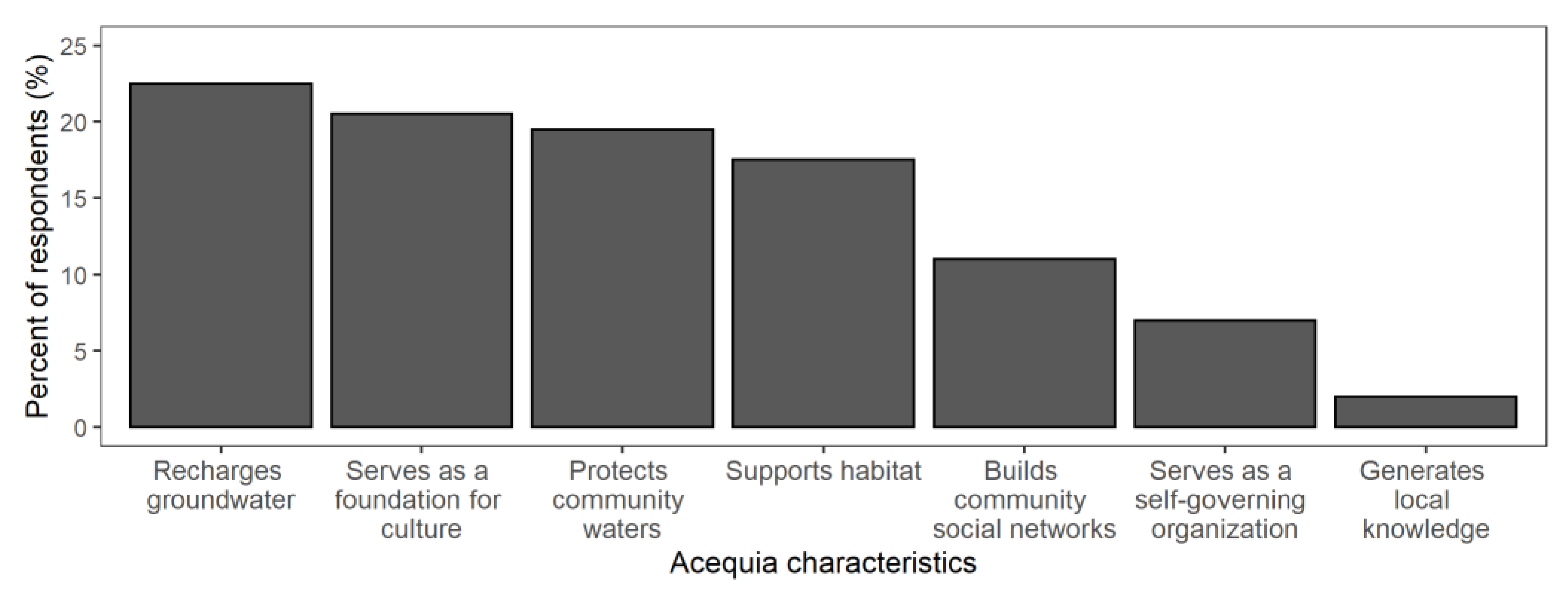This form of MAR reduces costs associated with infrastructure, piping, and energy given the gravity-driven water distribution [75]. This framework is naturally mirrored on a regional scale in northern New Mexico’s acequia networks. Acequia networks divert surface water through a system of (typically earthen) canals to fields for flood irrigation, where seepage occurs throughout time in the canals and application in the fields. Acequia irrigators greatly value these contributions to groundwater for the many environmental and water storage benefits the recharge provides (Figure 4). Acequias are not without their challenges, but they can serve as a model for sustainable, integrated water management that implicitly employs MAR and welcomes groundwater recharge as a benefit rather than an inefficiency [76].

Characterized by regular shallow aquifer recharge and flexible and dynamic water management that reflects equity and current environmental conditions, acequias offer several reasons why we should consider maintaining traditional irrigation systems in the face of climate change (Figure 5). In times of reduced surface water availability, acequia irrigators only irrigate smaller parcels of their total irrigated land and typically invest in deep rooted, drought-tolerant crops that can persist through growing seasons without much irrigation water application. Acequia communities have followed this model traditional flood irrigation model and persisted through drought for hundreds of years in northern New Mexico. However, when thinking about the future, the question then becomes: How should acequia communities adapt to meet reduced surface water availability and changing streamflow regime challenges that the current prolonged and unprecedented drought presents if traditional acequia irrigation practices are no longer sufficient?

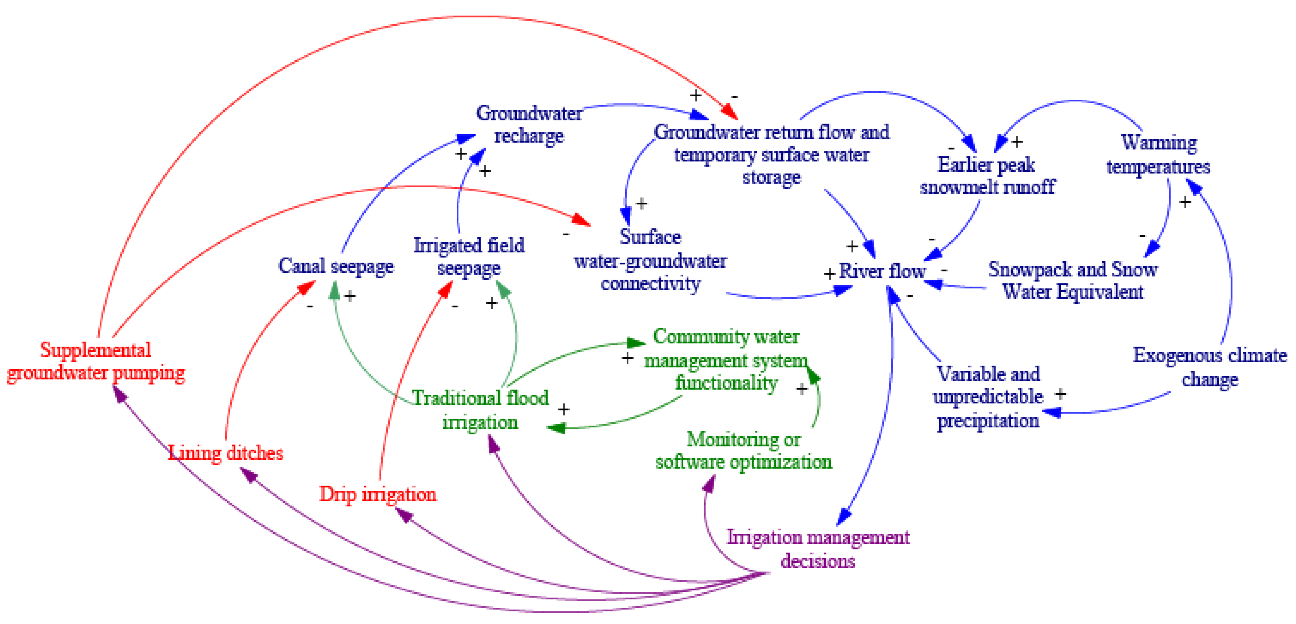
Traditional acequia operations are typically associated with resilience [77], but many acequia irrigators and managers are unsure of how sustainable certain adaptations are moving forward (e.g., lining earthen irrigation canals, switching from flood to drip irrigation, greater reliance on groundwater pumping) and the implications of any detrimental effects on groundwater levels (i.e., lowering the water table) which are ultimately connected to surface water availability (Figure 5). Lining irrigation ditches, switching from flood to drip irrigation, and supplemental groundwater pumping are commonly called into question by acequia community members which is why these adaptation strategies are highlighted in this paper. While these three strategies can be beneficial, lining ditches and drip irrigation reduce pathways for surface water to seep into the groundwater, and a growing reliance on groundwater pumping will negatively impact surface water and groundwater connectivity by lowering the water table (Figure 5). When used simultaneously in a region where baseflow is a crucial component of sustaining Rio Grande streamflow [56] and traditional acequia irrigation related recharge serves as delayed return flow [22], the reduction in groundwater recharge and the increase in groundwater pumping will negatively impact surface water availability for downstream users and begin propagating a cycle of maladaptation. It will be critical to prioritize traditional flood irrigation approaches and benefits such as groundwater recharge as much as possible when acequia communities or similar community-based irrigation systems are seeking solutions under conditions of reduced surface water availability.

It is important to distinguish between modernization of irrigation infrastructure and modernization of irrigation management. While lining ditches, switching to drip, and supplemental groundwater pumping focus on using surface water more efficiently through engineering and infrastructure improvements, water managers and irrigators must be provided with tools, resources, and information that enable efficient and adaptive water management and allocation. One example of this is real-time monitoring accessible through a web interface which has been shown to increase adaptive capacity indicators within the Rio Hondo acequia community [55]. With water scarcity only becoming a more pressing issue in the Southwest within the context of climate change, it will be critical to continue evaluating the adaptability of water management and agricultural production approaches, reflect findings in new and transformative policy, and ask ourselves if we should be modernizing infrastructure or management to avoid falling into the irrigation efficiency paradox trap [78,79].

A key element for the success of acequia and other community-based irrigation systems is community water management system functionality (see Figure 5). To have a functioning community water management system, there must first be a community to manage and use the water, so individuals must see value in acequias or acequia irrigation. When researchers explored capital gained within acequia communities, they found that only about 30% of family income was generated from acequia agriculture and that external income helped sustain acequia-irrigated properties and agriculture [80]. Surveys and interviews revealed that connection to land, water, and community were the values that drove acequia community members to respond to adverse circumstances (e.g., economic hardship, population growth, drought, increased development), demonstrating that acequia communities are founded and fueled by values within the moral economy rather than the typical market economy [30,59,80]. Therefore, identifying appropriate irrigation modernization recommendations must consider irrigation community motivations or values and be tailored toward enabling water management system functionality. While acequias foster long-term resilience, short-term vulnerabilities that impact acequia irrigation are surface water shortages. More work is needed to assess the specific impacts of changing irrigation regimes and technologies in acequia regions and identify adaptations that optimize groundwater recharge while also taking declining surface water availability into consideration.

5. Conclusions

In this study, we compared surface water and groundwater interactions and shallow aquifer response to irrigation events in two flood-irrigated forage grass fields located within the same acequia-irrigated valley in northern New Mexico, USA. Our results indicate that surface water and groundwater are tightly connected in this area, but variations in DP and groundwater response exists between land managers and fields due to differing flood irrigation scheduling and management. Additionally, while our results are consistent with previous water balance studies conducted in acequia-irrigated forage grass fields in northern New Mexico, this is the first paper to relate the findings from all the similar studies in the region since the first study was conducted in 2005. Because recharge acequia irrigation-related recharge eventually becomes delayed return flow to rivers [22], studies such as this are critical for determining how surface water and groundwater connectivity changes over time as it directly impacts surface water availability for downstream users [56]. We expect less DP will occur in acequia-irrigated fields if future climate change predictions and warming trends continue.

The DP and shallow groundwater recharge that occur as a byproduct of acequia flood irrigation are the exact management benefits needed for appropriate climate change adaptation. By maintaining recurring and consistent groundwater recharge, stream systems stay watered, which enables valley and regional cooperation between acequia-governing systems to continue. Alternatively, if acequia regions begin relying more heavily on groundwater pumping (for example), water tables would drop, making less water available in stream systems as surface water and groundwater become disconnected. These actions would propagate a cycle of maladaptation by undermining the hydrologic functions and community collaboration that make acequias so sustainable.

References

1. Barnett, T.P.; Adam, J.C.; Lettenmaier, D.P. Potential impacts of a warming climate on water availability in snow-dominated regions. Nature 2005, 438, 303–309. [Google Scholar] [CrossRef] [PubMed]
2. Harpold, A.; Brooks, P.; Rajagopal, S.; Heidbuchel, I.; Jardine, A.; Stielstra, C. Changes in snowpack accumulation and ablation in the intermountain west. Water Resour. Res. 2012, 48, 1–11. [Google Scholar] [CrossRef] [Green Version]
3. Clow, D.W. Changes in the timing of snowmelt and streamflow in Colorado: A response to recent warming. J. Clim. 2010, 23, 2293–2306. [Google Scholar] [CrossRef]
4. Payne, J.T.; Wood, A.W.; Hamlet, A.F.; Palmer, R.N.; Lettenmaier, D.P. Mitigating the effects of climate change on the water resources of the Columbia River basin. Clim. Change 2004, 62, 233–256. [Google Scholar] [CrossRef]
5. Hurd, B. Climate vulnerability and adaptive strategies along the Rio Grande/Rio Bravo border of Mexico and the United States. J. Contemp. Water Res. Educ. 2012, 149, 56–63. [Google Scholar] [CrossRef]
6. Elias, E.H.; Rango, A.; Steele, C.M.; Mejia, J.F.; Smith, R. Assessing climate change impacts on water availability of snowmelt-dominated basins of the Upper Rio Grande basin. J. Hydrol. Reg. Stud. 2015, 3, 525–546. [Google Scholar] [CrossRef]
7. Chavarria, S.B.; Gutzler, D.S. Observed changes in climate and streamflow in the Upper Rio Grande basin. J. Am. Water Resour. Assoc. 2018, 54, 644–659. [Google Scholar] [CrossRef] [Green Version]
8. Llewellyn, D.; Vaddey, S. West-Wide Climate Risk Assessment: Upper Rio Grande Impact Assessment Report; U.S. Department of the Interior, Bureau of Reclamation, Upper Colorado Region, Albuquerque Area Office: Albuquerque, NM, USA, 2013.
9. Bai, Y.; Fernald, A.; Tidwell, V.; Gunda, T. Reduced and earlier snowmelt runoff impacts traditional irrigation systems. J. Contemp. Water Res. Educ. 2019, 168, 10–28. [Google Scholar] [CrossRef]
10. Hurd, B.H.; Coonrod, J. Climate Change and Its Implications for New Mexico’s Water Resources and Economic Opportunities; Technical Report 45; New Mexico State University: Las Cruces, NM, USA, 2008. [Google Scholar]
11. Herrero, J.; Robinson, D.A.; Nogués, J. A regional soil survey approach for upgrading from flood to sprinkler irrigation in a semi-arid environment. Agric. Water Manag. 2007, 93, 145–152. [Google Scholar] [CrossRef]
12. Xu, X.; Huang, G.; Qu, Z.; Pereira, L.S. Assessing the groundwater dynamics and impacts of water saving in the Hetao Irrigation District, Yellow River basin. Agric. Water Manag. 2010, 98, 301–313. [Google Scholar] [CrossRef]
13. Magnuson, M.L.; Valdez, J.M.; Lawler, C.R.; Nelson, M.; Petronis, L. New Mexico Water Use By Categories 2015; New Mexico Office of the State Engineer: Santa Fe, NM, USA, 2019. [Google Scholar]
14. Fernald, A.; Tidwell, V.; Rivera, J.; Rodríguez, S.; Guldan, S.; Steele, C.; Ochoa, C.; Hurd, B.; Ortiz, M.; Boykin, K.; et al. Modeling sustainability of water, environment, livelihood, and culture in traditional irrigation communities and their linked watersheds. Sustainability 2012, 4, 2998–3022. [Google Scholar] [CrossRef] [Green Version]
15. Rivera, J.A.; Glick, T.F. The Iberian Origins of New Mexico’s Community Acequias. In Proceedings of the XIII Economic History Congress of the International Economic History Association, Buenos Aires, Argentina, 22–26 July 2002. [Google Scholar]
16. Rosenberg, A.; Guldan, S.; Fernald, A.G.S.; Rivera, J. Acequias of the Southwestern United States: Elements of Resilience in a Coupled Natural and Human System; College of Agricultural, Consumer and Environmental Sciences, New Mexico State University: Las Cruces, NM, USA, 2020. [Google Scholar]
17. Guldan, S.J.; Fernald, A.G.; Ochoa, C.G.; Tidwell, V.C. Collaborative community hydrology research in northern New Mexico. J. Contemp. Water Res. Educ. 2013, 152, 49–54. [Google Scholar] [CrossRef]
18. Sabie, R.P.; Fernald, A.; Gay, M.R. Estimating Land Cover for Three Acequia-irrigated Valleys in New Mexico using Historical Aerial Imagery between 1935 and 2014. Southwest. Geogr. 2018, 21, 36–56. [Google Scholar]
19. Fernald, A.G.; Cevik, S.Y.; Ochoa, C.G.; Tidwell, V.C.; King, J.P.; Guldan, S.J. River hydrograph retransmission functions of irrigated valley surface water-groundwater interactions. J. Irrig. Drain. Eng. 2010, 136, 823–835. [Google Scholar] [CrossRef]
20. Hamilton, P. Groundwater and surface water: A single resource. Water Environ. Technol. 2005, 17, 37–41. [Google Scholar]
21. Kendy, E.; Bredehoeft, J.D. Transient effects of groundwater pumping and surface-water-irrigation returns on streamflow. Water Resour. Res. 2006, 42, 1–11. [Google Scholar] [CrossRef]
22. Ochoa, C.G.; Fernald, A.G.; Guldan, S.J.; Tidwell, V.C.; Shukla, M.K. Shallow aquifer recharge from irrigation in a semiarid agricultural valley in New Mexico. J. Hydrol. Eng. 2013, 18, 1219–1230. [Google Scholar] [CrossRef]
23. Bouimouass, H.; Fakir, Y.; Tweed, S.; Leblanc, M. Groundwater recharge sources in semiarid irrigated mountain fronts. Hydrol. Process. 2020, 34, 1598–1615. [Google Scholar] [CrossRef]
24. Li, D. Quantifying water use and groundwater recharge under flood irrigation in an arid oasis of northwestern China. Agric. Water Manag. 2020, 240, 106326. [Google Scholar] [CrossRef]
25. Rotiroti, M.; Bonomi, T.; Sacchi, E.; McArthur, J.M.; Stefania, G.A.; Zanotti, C.; Taviani, S.; Patelli, M.; Nava, V.; Soler, V.; et al. The effects of irrigation on groundwater quality and quantity in a human-modified hydro-system: The Oglio River basin, Po Plain, northern Italy. Sci. Total Environ. 2019, 672, 342–356. [Google Scholar] [CrossRef]
26. Gutiérrez-Jurado, K.Y.; Fernald, A.G.; Guldan, S.J.; Ochoa, C.G. Surface water and groundwater interactions in traditionally irrigated fields in Northern New Mexico, U.S.A. Water 2017, 9, 102. [Google Scholar] [CrossRef]
27. Ochoa, C.G.; Fernald, A.G.; Guldan, S.J.; Shukla, M.K. Deep percolation and its effects on shallow groundwater level rise following flood irrigation. Am. Soc. Agric. Biol. Eng. 2007, 50, 73–82. [Google Scholar]
28. Fernald, A.G.; Baker, T.T.; Guldan, S.J. Hydrologic, riparian, and agroecosystem functions of traditional acequia irrigation systems. J. Sustain. Agric. 2007, 30, 147–171. [Google Scholar] [CrossRef]
29. Fernald, A.G.; Guldan, S.J. Surface water-groundwater interactions between irrigation ditches, alluvial aquifers, and streams. Rev. Fish. Sci. 2006, 14, 79–89. [Google Scholar] [CrossRef] [Green Version]
30. Fernald, A.; Guldan, S.; Boykin, K.; Cibils, A.; Gonzales, M.; Hurd, B.; Lopez, S.; Ochoa, C.; Ortiz, M.; Rivera, J.; et al. Linked hydrologic and social systems that support resilience of traditional irrigation communities. Hydrol. Earth Syst. Sci. 2015, 19, 293–307. [Google Scholar] [CrossRef] [Green Version]
31. Jakeman, A.J.; Barreteau, O.; Hunt, R.J.; Rinaudo, J.; Ross, A. Integrated Groundwater Management: Concepts, Approaches and Challenges; Springer Open: Berlin/Heidelberg, Germany, 2016. [Google Scholar]
32. Fuchs, E.H.; King, J.P.; Carroll, K.C. Quantifying disconnection of groundwater from managed-ephemeral surface water during drought and conjunctive agricultural use. Water Resour. Res. 2019, 55, 5871–5890. [Google Scholar] [CrossRef] [Green Version]
33. Hashemi, H.; Berndtsson, R.; Persson, M. Artificial recharge by floodwater spreading estimated by water balances and groundwater modelling in arid Iran. Hydrol. Sci. J. 2015, 60, 336–350. [Google Scholar] [CrossRef]
34. Ghasemizade, M.; Asante, K.O.; Petersen, C.; Kocis, T.; Dahlke, H.E.; Harter, T. An integrated approach toward sustainability via groundwater banking in the southern Central Valley, California. Water Resour. Res. 2019, 55, 2742–2759. [Google Scholar] [CrossRef]
35. Winter, T.C.; Harvey, J.W.; Franke, O.L.; Alley, W.M. Ground Water and Surface Water: A Single Resource; USGS Circular 1139; U.S. Geological Survey: Reston, VA, USA, 1999.
36. Jaber, F.H.; Shukla, S.; Srivastava, S. Recharge, upflux and water table response for shallow water table conditions in southwest Florida. Hydrol. Process. 2006, 20, 1895–1907. [Google Scholar] [CrossRef]
37. Scanlon, B.R.; Healy, R.W.; Cook, P.G. Choosing appropriate techniques for quantifying groundwater recharge. Hydrogeol. J. 2002, 10, 18–39. [Google Scholar] [CrossRef]
38. Fleming, W.M.; Rivera, J.A.; Miller, A.; Piccarello, M. Ecosystem services of traditional irrigation systems in northern New Mexico, USA. Int. J. Biodivers. Sci. Ecosyst. Serv. Manag. 2014, 10, 343–350. [Google Scholar] [CrossRef] [Green Version]
39. WRCC Taos, New Mexico-Climate Summary. Available online: https://wrcc.dri.edu/cgi-bin/cliMAIN.pl?nm8668 (accessed on 11 June 2021).
40. Cox, M. Applying a social-ecological system framework to the study of the Taos Valley irrigation system. Hum. Ecol. 2014, 42, 311–324. [Google Scholar] [CrossRef]
41. Sabu, S. Modeling Acequia Water Use in the Rio Hondo Watershed. Master’s Thesis, University of New Mexico, Albuquerque, NM, USA, March 2014. [Google Scholar]
42. United States Department of Agriculture, Natural Resources Conservation Service. Custom Soil Resource Report for Valdez, New Mexico; USDA-NRCS Web Soil Survey. Available online: http://websoilsurvey.nrcs.usda.gov/ (accessed on 28 July 2020).
43. United States Department of Agriculture, Natural Resources Conservation Service. Custom Soil Resource Report for Arroyo Hondo, New Mexico; USDA-NRCS Web Soil Survey. Available online: http://websoilsurvey.nrcs.usda.gov/ (accessed on 28 July 2020).
44. United States Department of Agriculture, Natural Resources Conservation Service. New Jersey Irrigation Guide; USDA-NRCS: Somerset, NJ, USA, 2005. [Google Scholar]
45. Samani, Z. Three simple flumes for flow measurement in open channels. J. Irrig. Drain. Eng. 2017, 143, 04017010-4. [Google Scholar] [CrossRef]
46. Blake, G.R.; Hartge, K.H. Bulk Density. In Methods of Soil Analysis, Part 1. Physical and Mineralogical Methods; Klute, A., Ed.; SSSA Book Ser. 5.1.; SSSA, ASA: Madison, WI, USA, 1986; pp. 377–382. [Google Scholar]
47. Gee, G.W.; Bauder, J.W. Particle-size Analysis. In Methods of Soil Analysis, Part 1. Physical and Mineralogical Methods; Klute, A., Ed.; SSSA Book Ser. 5.1.; SSSA, ASA: Madison, WI, USA, 1986; pp. 383–411. [Google Scholar]
48. Campbell Scientific, Inc. On-Line Estimation of Grass Reference Evapotranspiration with the Campbell Scientific Automated Weather Station; Application Note 4-D.; Campbell Scientific, Inc.: Logan, UT, USA, 1999. [Google Scholar]
49. Cevik, S.Y. A Long-Term Hydrological Model for the Northern Espanola Basin, New Mexico. Ph.D. Thesis, New Mexico State University, Las Cruces, NM, USA, December 2009. [Google Scholar]
50. Ochoa, C.G.; Fernald, A.G.; Guldan, S.J.; Shukla, M.K. Water movement through a shallow vadose zone: A field irrigation experiment. Vadose Zo. J. 2009, 8, 414–425. [Google Scholar] [CrossRef] [Green Version]
51. Moeser, C.D.; Chavarria, S.B.; Wootten, A.M. Streamflow Response to Potential Changes in Climate in the Upper Rio Grande Basin; USGS Scientific Investigations Report 2021-5138; U.S. Geological Survey: Reston, VA, USA, 2021.
52. Udall, B.; Overpeck, J. The twenty-first century Colorado River hot drought and implications for the future. Water Resour. Res. 2017, 53, 2404–2418. [Google Scholar] [CrossRef] [Green Version]
53. Rango, A. Snow: The real water supply for the Rio Grande basin. New Mex. J. Sci. 2006, 44, 99–118. [Google Scholar]
54. Lehner, F.; Wahl, E.R.; Wood, A.W.; Blatchford, D.B.; Llewellyn, D. Assessing recent declines in Upper Rio Grande runoff efficiency from a paleoclimate perspective. Geophys. Res. Lett. 2017, 44, 4124–4133. [Google Scholar] [CrossRef]
55. Conrad, L. Collaborative Community Hydrology: Integrating Stakeholder Engagement, Hydrology, and Social Indicators to Support Acequia Water Management in Northern New Mexico. Master’s Thesis, New Mexico State University, Las Cruces, NM, USA, May 2022. [Google Scholar]
56. Rumsey, C.A.; Miller, M.P.; Sexstone, G.A. Relating hydroclimatic change to streamflow, baseflow, and hydrologic partitioning in the Upper Rio Grande Basin, 1980 to 2015. J. Hydrol. 2020, 584, 124715. [Google Scholar] [CrossRef]
57. Cruz, J.J.; Fernald, A.G.; VanLeeuwen, D.M.; Guldan, S.J.; Ochoa, C.G. River-ditch flow statistical relationships in a traditionally irrigated valley near Taos, New Mexico. J. Contemp. Water Res. Educ. 2019, 168, 49–65. [Google Scholar] [CrossRef] [Green Version]
58. Fernald, A.; Guldan, S.J.; Sabie, R. Traditional Hydro-Cultural Water Management Systems Increase Agricultural Capacity and Community Resilience in Drought Prone New Mexico, USA. In Proceedings of the American Geophysical Union Fall Meeting, Washington, DC, USA, 10–14 December 2018. [Google Scholar]
59. Fernald, A.; Ochoa, C.G.; Guldan, S.J. Coupled Natural and Human System Clues to Acequia Resilience. In Acequias of the Southwestern United States: Elements of Resilience in a Coupled Natural and Human System; Rosenberg, A., Guldan, S., Fernald, A.G., Rivera, J., Eds.; New Mexico State University, College of Agricultural, Consumer and Environmental Sciences: Las Cruces, NM, USA, 2020; pp. 72–78. [Google Scholar]
60. Tolley, D.G.; Frisbee, M.D.; Campbell, A.R. Determining the importance of seasonality on groundwater recharge and streamflow in the Sangre de Cristo Mountains using stable isotopes. In Guidebook 66-Geology of the Las Vegas Area; Lindline, J., Petronis, M., Zebrowski, J., Eds.; New Mexico Geological Society Guidebook, 66th Field Conference; Geology of the Meadowlands: Las Vegas, NM, USA, 2015; pp. 303–312. [Google Scholar]
61. Li, X.; Fernald, A.G.; Kang, S. Assessing long-term changes in regional groundwater recharge using a water balance model for New Mexico. J. Am. Water Resour. Assoc. 2021, 57, 807–827. [Google Scholar] [CrossRef]
62. Olmstead, S.M. Climate change adaptation and water resource management: A review of the literature. Energy Econ. 2014, 46, 500–509. [Google Scholar] [CrossRef]
63. Barnett, J.; O’Neill, S. Maladaptation. Glob. Environ. Change 2010, 20, 211–213. [Google Scholar] [CrossRef]
64. Biddle, J.C.; Baehler, K.J. Breaking bad: When does polycentricity lead to maladaptation rather than adaptation? Environ. Policy Gov. 2019, 29, 344–359. [Google Scholar] [CrossRef]
65. Christian-Smith, J.; Levy, M.C.; Gleick, P.H. Maladaptation to drought: A case report from California, USA. Sustain. Sci. 2015, 10, 491–501. [Google Scholar] [CrossRef]
66. Torabi, E.; Dedekorkut-Howes, A.; Howes, M. Adapting or maladapting: Building resilience to climate-related disasters in coastal cities. Cities 2018, 72, 295–309. [Google Scholar] [CrossRef]
67. Haddad, B.M.; Merritt, K. Evaluating regional adaptation to climate change: The case of California water. In The Long-Term Economics of Climate Change; Hall, D.C., Howarth, R.B., Eds.; Elsevier Science: Amsterdam, The Netherlands, 2001; pp. 65–93. [Google Scholar]
68. McCaffrey, S.C. The need for flexibility in freshwater treaty regimes. Nat. Resour. Forum 2003, 27, 156–162. [Google Scholar] [CrossRef]
69. Jacobs, K.L.; Snow, L. Adaptation in the water sector: Science & institutions. Daedalus 2015, 144, 59–71. [Google Scholar] [CrossRef]
70. Sultana, P.; Thompson, P.M. Adaptation or conflict? Responses to climate change in water management in Bangladesh. Environ. Sci. Policy 2017, 78, 149–156. [Google Scholar] [CrossRef] [Green Version]
71. Cody, K.C. Flexible water allocations and rotational delivery combined adapt irrigation systems to drought. Ecol. Soc. 2018, 23, 47. [Google Scholar] [CrossRef]
72. Carlsson, L.; Berkes, F. Co-management: Concepts and methodological implications. J. Environ. Manag. 2005, 75, 65–76. [Google Scholar] [CrossRef]
73. Dillon, P.; Escalante, E.F.; Megdal, S.B.; Massmann, G. Managed Aquifer Recharge for Water Resilience. Water 2020, 12, 1846. [Google Scholar] [CrossRef]
74. Kwoyiga, L.; Stefan, C. Institutional feasibility of managed aquifer recharge in northeast Ghana. Sustainability 2019, 11, 379. [Google Scholar] [CrossRef] [Green Version]
75. Escalante, E.F.; Sebastián Sauto, J.S.; Gil, R.C. Sites and indicators of MAR as a successful tool to mitigate climate change effects in spain. Water 2019, 11, 1943. [Google Scholar] [CrossRef] [Green Version]
76. Pérez-Blanco, C.D.; Loch, A.; Ward, F.; Perry, C.; Adamson, D. Agricultural water saving through technologies: A zombie idea. Environ. Res. Lett. 2021, 16, 114032. [Google Scholar] [CrossRef]
77. Gunda, T.; Turner, B.L.; Tidwell, V.C. The influential role of sociocultural feedbacks on community-managed irrigation system behaviors during times of water stress. Water Resour. Res. 2018, 54, 2697–2714. [Google Scholar] [CrossRef]
78. Grafton, R.Q.; Williams, J.; Perry, C.J.; Molle, F.; Ringler, C.; Steduto, P.; Udall, B.; Wheeler, S.A.; Wang, Y.; Garrick, D.; et al. The paradox of irrigation efficiency. Science 2018, 361, 748–750. [Google Scholar] [CrossRef] [PubMed] [Green Version]
79. Bai, Y.; Langarudi, S.P.; Fernald, A.G. System dynamics modeling for evaluating regional hydrologic and economic effects of irrigation efficiency policy. Hydrology 2021, 8, 61. [Google Scholar] [CrossRef]
80. Mayagoitia, L.; Hurd, B.; Rivera, J.; Guldan, S. Rural community perspectives on preparedness and adaptation to climate-change and demographic pressure. J. Contemp. Water Res. Educ. 2012, 147, 49–62. [Google Scholar] [CrossRef]
Figure 1. Water balance field study sites: (a) F1 (located at 36°32′05.3″ N, 105°34′04.5″ W); (b) F2 (located at 36°31′47.8″ N, 105°41′00.7″ W) and the corresponding monitoring stations. Both fields are located in the Rio Hondo watershed in Taos County, northern New Mexico ((c) inset). Monitoring station locations were selected to most accurately represent average field conditions of the irrigated area while also considering landowner needs for equipment maneuverability while cutting hay.
Hydrology 09 00064 g001
Figure 2. Shallow groundwater levels for all monitoring wells, irrigation events (vertical gray lines), and DP estimates for the study sites: (a) F1; (b) F2 from early June 2020 through October 2021.
Hydrology 09 00064 g002
Figure 3. Boxplots created using daily averages of GWLF data from April 2021 through October 2021 visually comparing the medians, quartiles, and ranges of the three monitoring wells across both study fields.
Hydrology 09 00064 g003
Figure 4. When posed the question: “In addition to providing irrigation water for local uses, which of the following characteristics of acequias are most important to you?”, Rio Hondo Valley acequia community members (22.5%) reported groundwater recharge as the most valued attribute out of a variety of environmental, social, cultural, and governance options (n = 25). These data were collected as background information from adaptive capacity pre- and post-survey instruments distributed to the Rio Hondo acequia community. The final percent of respondents were averaged across the two surveys [55].
Hydrology 09 00064 g004
Figure 5. Causal loop diagram (CLD) showing the interactions and connections between environmental phenomena (blue), decision making (purple), adaptive management (green), and potentially maladaptive management (red) of acequia irrigation systems where traditional flood irrigation is assumed to only use surface water. Please note that the potentially maladaptive management options might be considered adaptive for other regions and irrigation regimes outside the scope of this paper.
Hydrology 09 00064 g005